Maximum Independent Set in Bipartite Graphs
Introduction
The title contains a lot of terms that should be explained separately before we start, given an undirected graph \(G = (V, E)\) we define the following terms:
- Independent Set (IS) : Subset of nodes \(U \subseteq V\) with the following propriety: For any two nodes \(u, v \in U\) nodes \(u, v\) are not adjacent ( There is no direct edge between nodes \(u\) and \(v\) ).
- Maximal Independent Set (MIS) : An independent set is maximal if no node can be added to it without violating the independence condition.
- Maximum Independent Set (MaxIS) : An independent set of maximum cardinality.
 |
|---|
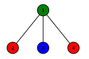
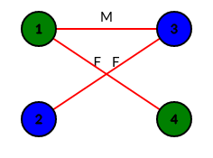
| Figure \(1\): Difference between IS, MIS and MaxIS |
Red nodes \((2, 4)\) are an IS, because there is no edge between nodes \(2\) and \(4\). However it’s not a MIS. Green node \((1)\) is a MIS because we can’t add any extra node, adding any node will violate the independence condition. Blue and red nodes \((2, 3, 4)\) are a MaxIS. It’s clear that there isn’t any other MIS with higher cardinality.
MIS can be found easily in \(O(V+E)\) we can use a sequential algorithm to find it, following these three simple steps:
- Initialize an empty set \(IS\).
- While \(V\) is not empty:
- Chose a random node \(u \in V\).
- Add \(u\) to the set \(IS\).
- Remove from \(V\) node \(u\) and all its neighbors.
- Return the set \(IS\).
However computing the MaxIS is a difficult problem, It is equivalent to the maximum clique on the complementary graph. Both problems are NP-hard. In this article we will consider a special case of graphs, the Bipartite Graphs as computing the MaxIS in this kind of graphs is much easier. So what is a Bipartite Graph?
\[\\\]Bipartite Graphs
A graph is called to be Bipartite if we can split the set of nodes \(V\) into two nonempty sets \(L, R\) and the following two conditions are true:
- For every two nodes \(u \in L\) and \(v \in L\) nodes \(u\) and \(v\) are not adjacent.
- For every two nodes \(u \in R\) and \(v \in R\) nodes \(u\) and \(v\) are not adjacent.
In 1916 Hungarian mathematician Dénes Kőnig published his works about the relation between the Minimum Vertex Cover (MVC) problem and the Maximum Cardinality Bipartite Matching (MCBM) problem in bipartite graphs. The theorem is called Kőnig’s line coloring theorem and it states:
In any bipartite graph, the number of edges in a Maximum matching equals the number of vertices in a minimum vertex cover.
We have presented many new terms that need to be explained, and we should also explain the relation between these new terms and the MaxIS term.
\[\\\]Minimum Vertex Cover (MVC)
A vertex cover is a set of nodes \(S\) such that for every edge \(e \in E\) at least one of its endpoints \((u, v) \in S\). A vertex cover in minimum if no other vertex cover has fewer vertices.
 |
|---|
| Figure \(2\): Red nodes are the MVC nodes |
Maximum Cardinality Bipartite Matching (MCBM)
Bipartite Matching is a set of edges \(M\) such that for every edge \(e_1 \in M\) with two endpoints \(u, v\) there is no other edge \(e_2 \in M\) with any of the endpoints \(u, v\). A matching is said to be maximum if there is no other matching with more edges.
Finding the MCBM can be done in polynomial time using many ways, next we will present a standard example problem, and talk about two solutions for this problem.
Motivation problem
A company has \(m\) different vacant jobs, \(n\) employees applied for these jobs, each employee applied for \(k_i\) jobs. Each employee can take exactly one job, and each job has only one vacant. Find a way to cover the most jobs.
Building the bipartite graph
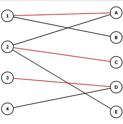
We will build a bipartite graph \(G = (V, E)\) with \(n+m\) vertices and \(\sum_{i=1}^{n} K_i\) edges. We add an edge between employee \(i\) and job \(j\), if the \(i_{th}\) employee applied for the \(j_{th}\) job. It’s clear that this graph is bipartite as there wont be edges between any two jobs or any two employees.
Consider this graph in the figure below, employees are numbered from \(1\) to \(4\) and jobs are classified by upper case letters \(A\) to \(E\). Red edges are the assignment of this bipartite graph.
 |
|---|
| Figure \(3\): MCBM in Bipartite Graph |
Max Flow Solution
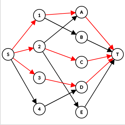
We can use Max Flow (I Will talk about it in much detail in future article) to solve the MCBM problem. This can be done by adding two extra dummy nodes to the graph, source node \(S\) and sink node \(T\). We add \(n\) directed edges with capacity \(1\) from \(S\) to nodes of the first set, also we add \(m\) directed edges with capacity \(1\) from every node of the second set to \(T\), we also set the capacity of the edges between the first set and second set to be equal to \(1\). When we run any Max Flow algorithm, like Edmonds Karp’s Algorithm or Dinic’s Algorithm we find the value of the max flow in the network, which is equivalent to the MCBM.
To find the actual matching assignment we check the flow value in every edge between nodes from the first set, and nodes from the second set. If the flow value in the edge \(e\) from node \(u\) to node \(v\) is \(1\). Then nodes \(u\) and \(v\) are matched together.
The complexity depends on the algorithm you use to find the Max Flow. In the worst case it’s \(O(n*m^2)\) if you use Edmonds Karp’s Algorithm and \(O(n^2*m)\) if you use Dinic’s Algorithm.
 |
|---|
| Figure \(4\): Flow Graph |
Augmenting Path Solution
MCBM problem can also be solved using the Augmenting Path Algorithm. Actually in programming contests it’s always better to use this method (in terms of implementation time and code length). An Augmenting Path is a path that starts from free (unmatched) vertex on the left set of the Bipartite Graph, alternate between a free edge (from the right side), a matched edge (from the left side), free edge (from the right side) and so on, until the path finally arrives on a free vertex on the right set of the Bipartite Graph. Claude Berge Lemma states that a matching \(M\) in graph \(G\) is maximum if and only if there is no more augmenting path in \(G\).
The algorithm finds an augmenting path using DFS traversal. There are a maximum of \(V\) augmenting paths in any graph, so the total complexity is \(O(V*E)\).
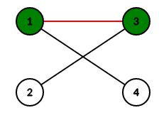
Lets explain how this algorithm finds augmenting paths, we start with free vertex \(1\) the algorithm will wrongly find augmenting path \((1-3)\), matching vertices \(1\) and \(3\).
In the next iteration we start from free vertex \(2\) from the left side, goes to vertex \(3\) via the free edge \((2-3)\), goes to vertex \(1\) via matched edge \((3-1)\), finally goes to vertex \(4\) via free edge \((1-4)\). Both vertices \(2, 4\) are free. Therefore the algorithm found augmenting path \((2-3-1-4)\). If we flip the edge status in this augmenting path free to matched and matched to free we get one more matching. The updated matching is shown in figure \(5_b.\)
 |
 |
|---|---|
| Figure \(5_a\): First iteration | Figure \(5_b\): Second iteration |
Below you can find the code to solve the MCBM problem using augmenting path algorithm.
vector<int>graph[MX];
bool vis[MX];
int match[MX];
bool dfs(int node){
	if(vis[node])return 0;
	vis[node] = 1;
	for(auto nx:graph[node]){
		if(match[nx]==-1 || dfs(match[nx])){
			match[node] = nx;
			match[nx] = node;
			return 1;
		}
	}
	return 0;
}
// inside main()
memset(match, -1, sizeof match);
while(1){
	memset(vis, 0, sizeof vis);
	bool cont = 0;
	for(int i=1;i<=n;i++){
		if(match[i]==-1)cont|=dfs(i);
	}
	if(cont==0)break;
}
int MCBM = 0;
for(int i=1;i<=n;i++){
	if(match[i]!=-1)MCBM++;
}
We should also mention that the MCBM problem can be solved in \(O(\sqrt{V} * E)\) using Hopcroft Karp’s algorithm, however I am not going to talk about it now, maybe in next articles I will talk about it in more details.
\[\\\]Back to the original problem
We have gone a little bit away from the original problem, started by the MaxIS problem and now we went through lot of different topics. Actually you cant really understand how to find the MaxIS in a bipartite graph without going through all these steps. There are two extra things we should mention before finishing this article. First thing states that:
The complement of a minimum vertex cover in any graph is the maximum independent set.
In conclusion we can say, in bipartite graphs solving the NP-Hard MaxIS can be reduced to solving NP-Hard MVC problem, this also can also be reduced to solving the polynomial MCBM problem.
\(\\\)
Last piece of the jigsaw
The last missing piece is about finding the actual nodes of the MaxIS. First we solve the MCBM problem and find the set of edges \(M\) that form the maximum matching for the graph. To find the nodes of the MVC we do the following:
- Give orientation to the edges, matched edges start from the right side of the graph to the left side, and free edges start from the left side of the graph to the right side.
- Run DFS from unmatched nodes of the left side, in this traversal some nodes will become visited, others will stay unvisited.
- The MVC nodes are the visited nodes from the right side, and unvisited nodes from the left side.
Prof
For each edge \(e \in M\) we should either take its left endpoint or its right endpoint, but not both, if we take both of its endpoints we will end up by vertex cover of size greater than the MCBM as each edge should be covered.
Lets prove that all visited nodes of the right side are part of the MVC. When we start from unmatched node from the left side, we can only go by a free edges to the right side, this node from the right side is clearly incident to some edge \(e \in M\) (otherwise we would have matched these two nodes together). As the unmatched node from the left side is not part of the MVC then we must take the right side node. Next we go back to the left side using a matched edge. As the right side of this edge is part of the MVC we cant take this node (check the previous paragraph). And so on until we finish traversing the graph.
After the traversal is over, we can split the graph into these four sets:
- \(V_L\) Visited nodes from the left side.
- \(U_L\) Unvisited nodes from the left side.
- \(V_R\) visited nodes from the right side.
- \(U_R\) Unvisited nodes from the right side.
We have proven that \(V_R\) are defiantly part of the MVC and \(V_L\) are defiantly not part of the MVC. For the \(U_L\) and \(U_R\) it turns out that all the \(U_L\) nodes are defiantly part of the MVC and \(U_R\) are defiantly not part of the MVC. To prove this, just consider the left side as right side, and the right side as left side for the unvisited nodes, and do the same as before.
After finding the MVC nodes, you just have to take its complement to find the MaxIS nodes, and you are done.
So eventually we can write:
\[MVC = V_R \cup U_L.\] \[MaxIS = V \setminus MVC.\]Conclusion
Through this article we went across different topics, started with introducing the Independent Set term and explaining its meaning, along with the Maximal and Maximum Independent Set terms, next up we moved to talk about Bipartite graphs, and mentioned Kőnig’s theorem, after that we talked about the Minimum Vertex Cover problem and the Maximum Cardinality Bipartite Matching problem, we mentioned a classical MCBM problem and showed two methods of solving it, the Max Flow method, and the Augmenting Paths algorithm. Later we went back to the original MaxIS problem, and explained the relation between MVC and MaxIS. Finally through the prof of Kőnig’s theorem we showed how to find the nodes of the MVC and eventually the nodes of the MaxIS. You can find the full code for the solution of the motivation problem here.
Practice Problems
Extra reading + List of acronyms
- IS Independent Set.
- MIS Maximal Independent Set.
- MaxIS Maximum Independent Set.
- Kőnig’s Theorem.
- MVC Minimum Vertex Cover.
- MCBM Maximum Cardinality Bipartite Matching
- Max Flow.
I hope you liked this article, please stay tuned for more.