Combinatorial Games

The game is said to be Combinatorial if it satisfies the following conditions:

The game is played between two players, we will call them Alice and Bob.
The two players alternate playing, Alice plays first.
We can define two sets \(F_1\) and \(F_2\) of possible moves for each player, these sets are usually finite, based on these two sets we can classify combinatorial games into:
- Combinatorial impartial games this happens when \(F_1 = F_2\), this means both players have the same options of moving from each position.
- Combinatorial partizan games this happens when \(F_1\ne F_2\), this includes games like chess or checkers in which one player moves the white pieces, and the other player moves the black pieces.
There is an end position of the game, usually called the terminal position. In normal play rule the player making the last move wins the game, in misère play rules the player making the last move loses the game.
The game always ends after some finite number of moves.

P-positions and N-positions

Every position in the game can be either Previous or Next. previous positions are wining for the previous player (the player who just moved), and next positions are wining for the next player to move. We can find P and N positions using these rules:

All terminal positions are P-positions.
From every N-position there is at least one move to a P-position.
From every P-position, every move is to an N-position.

Motivation Problem

Alice and Bob are playing a game, there are \(N\) coins, Alice starts first and they alternate taking these coins, in each turn the player can take at least one coin, and up to \(3\) coins. The game is played in normal play rules (player taking the last coin wins the game). Let’s start by finding P and N positions of the game: The terminal position is when there are no coins left and \(N=0\) this is a P-position. When \(N=1, 2, 3\) the player to play can take all the remaining coins and reach \(N=0\) position, which is a P-position. Therefore all these positions are N-positions. When \(N=4\) the possible moves are:

Take one coin to position \(N=3\) which is an N-position.
Take two coins to position \(N=2\) which is an N-position.
Take three coins to position \(N=1\) which is an N-position.

Therefore \(N=4\) is a P-position.

When \(N=5, 6, 7\) the player to play can take \(1, 2, 3\) coins respectively reaching \(N=4\) position, which is a P-position. Therefore all these positions are N-positions. The process repeats with this pattern PNNNPNNNP… Eventually the position is P-position if \(N \bmod 4=0\).

Nim Game

The most famous take-away game is the nim game, The game can be described as following: Alice and Bob are playing a game, there are \(N\) piles of coins, every pile contain \(a_i\) coins. Alice starts first and they alternate taking these coins, each move consists of selecting nonempty pile and removing at least one coin from it. The game is played in normal play rules (player taking the last coin wins the game).

Nim-sum

The nim-sum of two non-negative integers is their addition without carry in base 2. Described as: Let \(X(x_m x_{m-1} ... x_0)_2\) and \(Y(y_m y_{m-1} ... y_0)_2\) be two non-negative integers writing in base 2. And let \(Z(z_m z_{m-1} ... z_0)_2\) be their nim sum, \(Z\) can be written as:

\[Z(z_m z_{m-1} ... z_0)_2 = X(x_m x_{m-1} ... x_0)_2 \oplus Y(y_m y_{m-1} ... y_0)_2 .\] \[z_k = x_k + y_k \bmod 2 .\]

Let’s take this example:

\[X = 12_{10} = 01100_2\] \[Y = 23_{10} = 10111_2\] \[Z = 27_{10} = 11011_2\]

Bouton Theorem

A position \((x_1, x_2, ... x_n)\) is a P-position if and only if the nim-sum of it’s components is zero, \(x_1 \oplus x_2 \oplus .... \oplus x_n = 0.\)

Let’s take these examples:

\[x_1 = 12_{10} = 1100_2\] \[x_2 = 10_{10} = 1010_2\] \[x_3 = 13_{10} = 1101_2\]

\(nim\) - \(sum = 11_{10} = 1011_2 \ne 0\), So this is a N-position.

\[x_1 = 10_{10} = 1010_2\] \[x_2 = 10_{10} = 1110_2\] \[x_3 = \,\,\,4_{10} = 0100_2\]

\(nim\) - \(sum = 0_{10} = 0000_2 = 0\), So this is a P-position.

Proof

Let \(\mathcal{P}\) donate the set of nim positions with zero nim-sum, and let \(\mathcal{N}\) be the set of nim positions with non zero nim-sum.

The only terminal position is \((0, 0, ... , 0)\) it’s clear that this position belongs to \(\mathcal{P}.\)
From every position in \(\mathcal{N}\) there is one move to a position in \(\mathcal{P}.\) To construct this move, we look at the most significant bit with odd number of \(1's\). Change any number having this bit turned on to another number to make all the bits occur even number of times. This move is legal because the most significant bit in this number will become zero, so eventually the number of coins in that pile will decrease.
From every position in \(\mathcal{P}\), every move is to a position in \(\mathcal{N}.\) Let’s prove that there isn’t any move from any position from \(\mathcal{P}\) to another \(\mathcal{P}\) position. If \((x_1, x_2, ..., x_n)\) is in \(\mathcal{P}\) and \(x_1\) changes to \({x_1}^{\prime} < x_1\) Then we can’t have \(x_1 \oplus x_2 \oplus .... \oplus x_n = 0 = x_1^{\prime} \oplus x_2 \oplus .... \oplus x_n = 0\) as this means \(x_1 = x_1^{\prime}.\)

Bouton’s Theorem gives us a way to find the number of possible moves from a N-position, this is the number of \(1's\) in the most significant bit with odd number of \(1's\). Note that this number is always odd.

Bouton’s Theorem defines a way to play misère nim optimally, as long as there are at least two piles of size greater than \(1\) play the game as normal nim, when your turn comes and there is exactly one pile of size greater than \(1\) then you should either take this whole pile, or just leave \(1\) coin int it, whichever leaves an odd number of ones remaining.

Games and graphs

We will start by representing games using directed graphs. Every position in the game can be represented as a vertex in directed graph, the set of moves from some position to another are the edges of the directed graph. More formally we can represent the game using graph \(G(X, F)\). Where \(X\) is nonempty set of vertices(positions), and \(F\) is a function that gives for each \(x \in X\) a subset \(F(x) \subseteq X.\) Where \(F(x)\) represents the positions a player can move from \(x\), called the followers of \(x.\) If \(F(x)\) is empty then position \(x\) is a terminal position.

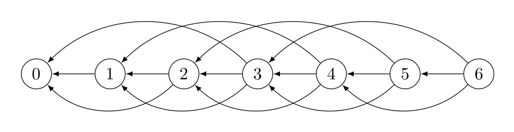
Let’s take the subtraction problem discussed before as an example, in this problem \(X = {0, 1, 2, .... ,N}\). Empty pile \(N=0\) is the terminal position, \(F(0) = \emptyset\), \(F(1) = \{0\}\), \(F(2) = \{0, 1\}\), \(F(n) = \{n-1, n-2, n-3\}\) for \(3 \le n \le N\). The corresponding graph is shown in figure \(1\) below.


Figure 1: subtraction game graph for \(N=6\)

Sprague-Grundy Function

Sprague-Grundy Function of a graph \(G(X, F)\) can be defined as:

\[g(x) = min\{n\ge 0 :n\ne g(y), y\in F(x)\}.\]

In other words \(g(x)\) is the minimal non-negative number found in the follows of \(x.\) This is also called the minimal excludant or mex function, so we can write:

\[g(x) = mex\{g(y) : y\in F(x)\}.\]

Sprague-Grundy function can be found using inductive technique, we start from terminal vertices, since \(F(x) = \emptyset\) for these vertices then \(g(x) = 0.\) For all vertices \(y\) such that there is a terminal vertex \(x \in F(y)\) we write \(F(y) = 1.\) In general we can write:

If \(x\) is terminal vertex then \(g(x) = 0.\)
If \(g(x) = 0\) then for all other vertices \(y\) such that \(x \in F(y)\), \(g(y) \neq 0.\)
If \(g(x) \neq 0\) There is at least one vertex \(y \in F(x)\) such that \(g(x)=0.\)

Sprague-Grundy Function gives us a lot of details about the game more than just finding N and P positions, Using Sprague-Grundy Theorem we can analyze the sums of the game, and gives us a way to understand games in these graphs.

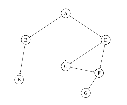
Let’s check the graph in Figure \(2\) below, and the corresponding Sprague-Grundy function values.


Figure 2: Sprague-Grundy function

vertex \(x\)	\(A\)	\(B\)	\(C\)	\(D\)	\(E\)	\(F\)	\(G\)
\(g(x)\)	3	1	0	2	0	1	0

Graph games that end after finite number of moves are called progressively bounded graphs, in this graphs for every starting position \(x_0\) any path in the graph have a finite length, this ensures the ending condition of the game, and eliminates cycles, eventually eliminating ties in the game, graph in Figures \(1\) and \(2\) above is an example of such graphs.

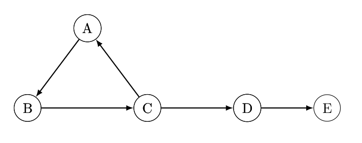
In graphs with cycles the SG-Function may not exist, even if it exists finding it would be hard, or even there might not be a winning strategy for these games, let’s take the graph in figure \(3\) below as an example.


Figure 3: Graph with cycle

In the graph above \(g(E) = 0\), \(g(D) = 1\). However we can’t define the SG-Function for other nodes, when player \(1\) is at node \(C\) choosing to make a move to node \(D\) will make him lose, so he will make the move to node \(A\), player \(2\) will make the move to node \(B\), player \(1\) will then make the move to node \(C\). Now it’s the second player to move at node \(C\), again moving to node \(D\) will make him lose, so he will move to node \(A\). The game get stuck in this cycle and and eventually the game never ends.

Sum of Combinatorial Games

Several combinatorial games can be combined together to make a new combinatorial game, in every game we define it’s corresponding graph \(G_i(X_i, F_i)\), a starting position \(x_0\) is defined at each game and in every turn a player chooses one of these games and makes a legal move in this game, leaving other games untouched, the game ends when terminal positions are reached in all these games. This game is called (disjunctive) sum of the given games.

Definition

For a given set of \(n\) progressively bounded graphs \(G_i(X_i, F_i)\) for \(1 \le i \le n\). We can combine these graphs in a new graph \(G = \sum\limits_{i=1}^{i=n} G_i\). The set of vertices \(X\) is the cartesian product \(X = \prod\limits_{i=1}^{i=n} X_i\). This is the set of all n-tuples \((x_1,x_2,\dots,x_n)\) such that \(x_i \in X_i\), for a vertex \(x = (x_1,x_2,\dots,x_n)\) we define the followers of vertex \(x\):

\[\begin{aligned} F(x) = F(x_1, x_2,\dots,x_n) = &F_1(x_1) \times \{x_2\} \times \dots \times\{x_n\} \\ &\cup \; \{x_2\} \times F_2(x_2) \times \dots \times \{x_n\} \\ &\cup \; \dots \\ &\cup \; \{x_1\} \times \{x_2\} \times \dots \times F_n(x_n) \end{aligned}\]

If each of the \(n\) graphs is progressively bounded then the resulting graph \(G\) is also progressively bounded, nim-game with \(n\) piles is an example of such graph, where each of the piles can be considered a progressively bounded graph, and all the graph of all the games is the sum of these graphs.

Sprague-Grundy Theorem

If \(g_i\) is the SG-Function of \(G_i\) Then \(G = \sum\limits_{i=1}^{i=n} G_i\) has SG-Function:

\[g(x_1,x_2,\dots,x_n) = g_1(x_1) \oplus g_2(x_2) \oplus \dots \oplus g_n(x_n)\]

This means that every progressively bounded impartial game is equivalent to a nim-pile with size equal to its SG-Function value.

Motivation Problem

A nawl is an imaginary chess piece that has the following set of moves: \(F(i, j) = \{(i+1, j), (i, j+1), (i+1, j+1)\}.\)A move is said to be legal if it doesn’t move the nawl out of the chessboard, and if the new cell is not blocked (multiple nawls can share the same cell). Alice and Bob are playing a game with nawls, the chessboard size is \(n\times n\), initially \(k\) nawls are placed in the chessboard, no nawl is placed in a blocked cell, in each cell the player in his turn makes a legal move, the player to make the last move wins the game, if the players play optimally, who wins the game?

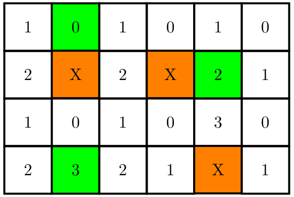
To solve this problem we will use the SG-Theorem, let’s first solve the problem for just one nawl, then use the combinatorial games sum property to sole the bigger game. Let’s take this example and calculate the SG-Function values for every position of the game, orange cells are blocked cells, and green cells are cells with a nawl.


Figure 4: SG-Theorem

According to SG-Theorem the nim-sum of this game is equal to \(2\oplus 0 \oplus 3 = 1 \neq 0\) so this is a winning position for the first player, the playing strategy is same as the nim-game, In the example above the first move in the optimal strategy would be to move the nawl is cell \((2, 1)\) to cell \((3, 1)\) as this makes the total nim-sum equal to zero, which is a P position.

Conclusion

In this article I went through lots of topics related to game theory, first I started by defining combinatorial games, and gave a simple subtraction game as an example explaining how to find P and N positions, Next on I introduced Nim-games and gave a proof how Bouton’s Theorem can be used to play the game. Later I showed how to represent games on directed graphs, and talked about Sprague-Grundy Function, finally I have mentioned how to use SG-Theorem to play games on graphs defined by the sum of many combinatorial games and gave a brief example about the theorem. Sprague-Grundy Theorem can be used to solve many problems related to competitive programming, in this article I just wanted to show and explain lots of concepts, maybe in a next article I will focus more on explaining different problems and how to solve them.

I hope you liked this article, please stay tuned for more.